Density dependent change

class: center, middle, inverse, title-slide

.title[
# Density dependent change
]
.author[
### Christopher Moore
]

---

# Creating a density-dependent model, au Français
![VerhulstImage](Wk03_DensDep_files/Verhulst.png)
---
# Creating a density-dependent model, translated

*If `$p$` is the population, then `$dp$` is an infinitesimally small increase that is received in a very short period of time `$dt$`. If the population increase by geometric progression, we would have the equations `$\frac{dp}{dt} = mp$`. However, as the rate of population growth is slowed by the very increase in the number of inhabitants, we must subtract from `$mp$` an unknown function of `$p$`, so that the formula to be integrated can be written as*
`$$\frac{dp}{dt} = mp - \varphi (p)$$`
*The simplest hypothesis that can be made on the form of the function `$\varphi$` is to suppose that `$\varphi (p) = np^2$`.*
---
# The logistic model: a balance of forces
Most generally, we wish model population growth with two functions that capture two biological phenomena, growth and crowding.
--
`$$\frac{\Delta N}{\Delta t} = f(N),$$` 
with `$f(N)$` describing growth and crowding:

`$$f(N) = \text{growth} - \text{crowding}.$$`
--

Let growth be `$rN$` and crowding be `$\alpha N^2$`, to give us
`$$\frac{\Delta N}{\Delta t} = rN - \alpha N^2$$`
--
In continuous and discrete time the logistic equations are respectively:  
`$$\begin{align}
\frac{dN}{dt} &= rN - \alpha N^2 \\
N_{t+1} &= \lambda N_t - \alpha N_t^2
\end{align}$$`

---
# Births and deaths in the logistic model
(I'm only describing continous time, but it's analagous in discrete time) A generalized way of writing a more mechanistic model of births and deaths into the logisitc model is respectively by the use of functions of `$N$`, `$B(N)$` and `$D(N)$`:
--
`$$\frac{dN}{dt} = B(N) - D(N)$$`
--
Let's say that both per-capita births and death rates linearly decrease as a function of density, `$N$`. So, we can write:
--
`$$\frac{dN}{dt} = (bN - \mu N^2) - (dN - \nu N^2)$$`
--
Linearity becomes clear when we write this as *per-capita* by dividing both sides by `$N$`:
`$$\frac{1}{N}\frac{\mathrm{d}N}{\mathrm{d}t} = (b - \mu N) - (d - \nu N)$$`
---
class: inverse, center, middle
<a href="https://imgflip.com/i/25ds0b"><img src="https://i.imgflip.com/25ds0b.jpg" title="made at imgflip.com"/></a>

---
# We have (a) model(s)—let's do all of the things!
* Analyze it!
  * Simulate it
  * Solve it
  * Find equilibria (long-term behavior)
  * Determine stability (behavior if perturbed)
* Visualize it!
  * Plot a time series
  * Plot population size `$(N)$` and population growth `$\left(\frac{dN}{dt}\right)$`
  * Plot population size `$(N)$` and per-capita growth `$\left(\frac{1}{N}\frac{dN}{dt}\right)$`
  
---
# Analyze it!: simulation
.pull-left[
Exactly what you did yesterday:
![](Wk03_DensDep_files/figure-html/unnamed-chunk-1-1.png)
]

--
.pull-right[
But also vary parameters (here, `$r$`):
![](Wk03_DensDep_files/figure-html/many.log-1.png)
]

---
#Analyze it!: solve it
For the `$r\text{-}\alpha$` logistic equation:
`$$N(t) = \frac{rN(0)e^{rt}}{r + \alpha N(0)\left(e^{rt} - 1\right)}$$`

For the `$K$` logistic equation:
`$$N(t) = \frac{KN(0)e^{rt}}{K + N(0)\left(e^{rt} - 1\right)}$$`
--

** This will be the final analytical solution in this class 😥 **

---
#Analyze it!: finding equlibria

The continuous logistic
`$$\begin{align}\frac{\mathrm{d}N}{\mathrm{d}t} &= rN - \alpha N^2 \\
0 &= rN - \alpha N^2 \\
0 &= N\left(r - \alpha N\right) \\
N^* &= 0 \\
0 &= r - \alpha N\\
\alpha N &= r \\
N^* &= \frac{r}{\alpha}
\end{align}$$`

---
#Analyze it!: finding equlibria

The discrete logistic
`$$\begin{align}
N_{t+1} &= \lambda N_t - \alpha N_t^2 \\
N_t &= \lambda N_t - \alpha N_t^2 \\
0 &= \lambda N_t - \alpha N_t^2 - N_t \\
0 &= N_t \left(\lambda - \alpha N_t - 1 \right) \\
N^* &= 0 \\
0 &= N_t \left(\lambda - \alpha N_t - 1 \right) \\
0 &= \lambda - \alpha N_t - 1 \\
\alpha N_t &= \lambda - 1 \\
N^* &= \frac{\lambda - 1}{\alpha}
\end{align}$$`

---
# Analyze it!: perturbation
Perturb the equilibira! Actually, we'll cover more of this in Ch. 4, *Dynamics.*

---
# Visualize it!: time series

```r
logistic <- function(t, y, p) {
  N <- 1.5*y - 0.15*y^2
  return(list(N))
}
out <- ode(y = 0.01, times = seq(0, 10, 0.01), parms = NA, func = logistic)
par(mar = c(4, 4, 0.1, 0.1), oma = c(0, 0, 0, 0))
plot(x = out[,1], y = out[,2], las = 1, xlab = "Time", ylab = "Density (N)", type = "l", lwd = 2)
```

![](Wk03_DensDep_files/figure-html/unnamed-chunk-2-1.png)

---
# Visualize it!: population growth and density

```r
logistic <- function(t, y, p) {
  N <- 1.5*y - 0.15*y^2
  return(list(N))
}
out <- ode(y = 0.01, times = seq(0, 10, 0.01), parms = NA, func = logistic)
par(mar = c(4, 4, 0.1, 0.1), oma = c(0, 0, 0, 0))
len.out <- nrow(out)
plot(x = out[1:(len.out-1),2], y = (out[2:len.out,2] - out[1:(len.out-1),2]), las = 1, xlab = "Density (N)", ylab = "Population growth (dN/dt)", type = "l", lwd = 2)
```

![](Wk03_DensDep_files/figure-html/unnamed-chunk-3-1.png)

---
# Visualize it!: per-capita growth and density

```r
logistic <- function(t, y, p) {
  N <- 1.5*y - 0.15*y^2
  return(list(N))
}
out <- ode(y = 0.01, times = seq(0, 10, 0.01), parms = NA, func = logistic)
par(mar = c(4, 4, 0.1, 0.1), oma = c(0, 0, 0, 0))
len.out <- nrow(out)
plot(x = out[1:(len.out-1),2], y = (out[2:len.out,2] - out[1:(len.out-1),2])/out[1:(len.out-1),2], las = 1, xlab = "Density (N)", ylab = "Per calita growth (dN/dt/N)", type = "l", lwd = 2)
```

![](Wk03_DensDep_files/figure-html/unnamed-chunk-4-1.png)

---
# Discrete-time density dependence

--
Hassel (also Bleasdale and Nedler) model:
`$$N_{t+1} = \frac{\lambda N_t}{\left(1 + \alpha N_t\right)^b}$$`

--
Beverton and Holt (same as Hassel when `$b = 1$`):
`$$N_{t+1} = \frac{\lambda N_t}{\left(1 + \alpha N_t\right)}$$`
--
The Ricker equation:
`$$N_{t+1} = N_t \exp\left(r\left(1 - bN_t\right)\right)$$`

---
# Analyze it!: simulation

.pull-left[
Choosing the Hassell model:
![](Wk03_DensDep_files/figure-html/unnamed-chunk-5-1.png)
]

--
.pull-right[
But also vary parameters (here, `$b$`):
![](Wk03_DensDep_files/figure-html/many.disc.log-1.png)
]

---
# Analyze it!: solve it and find equilibria

1. No analytical solutions
2. We can find equilibira for some!
   - For discrete-time equations, set `$N_{t + 1} = N^*$` and `$N_t = N^*$`, and solve for `$N^*$`
   - E.g.,

`$$\begin{align}
N_{t+1} &= \frac{\lambda N_t}{1 + \alpha N_t} =  \\
N^* &=\frac{\lambda N^*}{1 + \alpha N^*} \\
N^* &= 0,~\text{Equilibrium 1} \\
1 &= \frac{\lambda}{1 + \alpha N^*} \\
1 + \alpha N^* &= \lambda \\
\alpha N^* &= \lambda - 1 \\
N^* &= \frac{\lambda - 1}{\alpha},~\text{Equilibrium 2}\\
\end{align}$$`

---
# Analyze it!: perturb equilibira
Again, more on this in a few weeks.

---
# Visualize it!: time series

```r
Hassell <- function(t, y, p) {
  Nt <- y
  lambda <- p["lambda"]
  alpha <- p["alpha"]
  b <- p["b"]
  Nt1 <- lambda*Nt/((1 + alpha*Nt)^b)
  return(list(Nt1))
}
Hassell.parms <- c(lambda = 1.5, alpha = 2, b = 0.5)
out <- ode(y = 0.01, times = seq(0, 25, 1), parms = Hassell.parms, func = Hassell, method = "iteration")
par(mar = c(4, 4, 0.1, 0.1), oma = c(0, 0, 0, 0))
plot(x = out[,1], y = out[,2], las = 1, xlab = "Time", ylab = "Density (N)", type = "p", lwd = 2, pch = 16)
  segments(x0 = out[,1][-nrow(out)], y0 = out[,2][-nrow(out)], x1 = out[,1][-1], y1 = out[,2][-nrow(out)], lwd = 2)
```

---
# Visualize it!: time series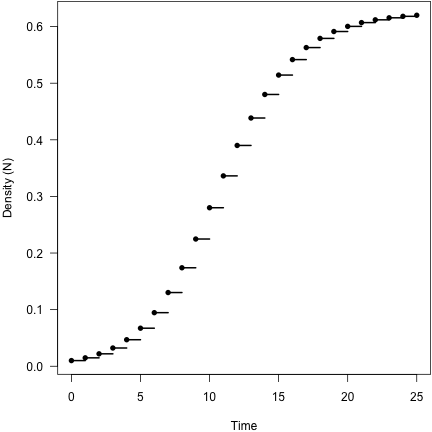
![](Wk03_DensDep_files/figure-html/unnamed-chunk-7-1.png)

---
# Visualize it!: population growth and density

```r
Hassell <- function(t, y, p) {
  Nt <- y
  lambda <- p["lambda"]
  alpha <- p["alpha"]
  b <- p["b"]
  Nt1 <- lambda*Nt/((1 + alpha*Nt)^b)
  return(list(Nt1))
}
Hassell.parms <- c(lambda = 1.5, alpha = 2, b = 0.5)
out <- ode(y = 0.001, times = seq(0, 40, 1), parms = Hassell.parms, func = Hassell, method = "iteration")
Hassell.out <- out[-1,2] - out[-nrow(out),2]
plot(x = out[1:(nrow(out)-1),2], y = Hassell.out, las = 1, xlab = "Density (N)", ylab = bquote("Population growth N"[t+1]-"N"[t]), type = "l", lwd = 2)
```

---
# Visualize it!: population growth and density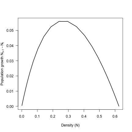

![](Wk03_DensDep_files/figure-html/unnamed-chunk-9-1.png)

---
# Visualize it!: per-capita growth and density

```r
Hassell <- function(t, y, p) {
  Nt <- y
  lambda <- p["lambda"]
  alpha <- p["alpha"]
  b <- p["b"]
  Nt1 <- lambda*Nt/((1 + alpha*Nt)^b)
  return(list(Nt1))
}
Hassell.parms <- c(lambda = 1.5, alpha = 2, b = 0.5)
out <- ode(y = 0.001, times = seq(0, 40, 1), parms = Hassell.parms, func = Hassell, method = "iteration")
Hassell.out <- (out[-1,2] - out[-nrow(out),2])/out[-1,2]
plot(x = out[1:(nrow(out)-1),2], y = Hassell.out, las = 1, xlab = "Density (N)", ylab = bquote("Population growth N"[t+1]-"N"[t]/"N"[t]), type = "l", lwd = 2)
```

---
# Visualize it!: per-capita growth and density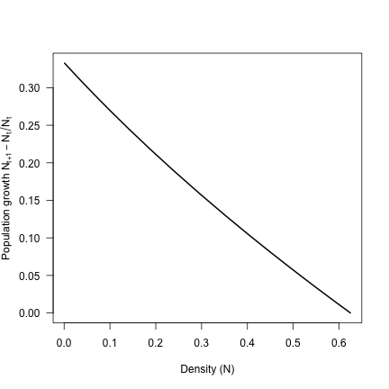

![](Wk03_DensDep_files/figure-html/unnamed-chunk-11-1.png)