class: center, middle, inverse, title-slide .title[ # Disease dynamics ] .author[ ### Christopher Moore ] --- # Diversity of disease models There are many different models of disease dynamics, given the *enormous* diversity of pathogen, vector, and host life histories. (Notice that we are only considering the dynamics of the host and not the pathogen.) As some examples: -- I. Susceptibles become infected, and remain infected for their lives -- II. Susceptibles become infected, fight off the disease, and again become susceptible -- III. Susceptibles become infected, fight off the disease, and become resistant to subsequent infection -- IV. Some diseases include a latent period before making the infected infectious -- V. Some diseases can exist post-infected "carriers" that are no longer harmed, but can be indefinitely infectious -- VI. Some diseases are maternally inherited -- VII. Some diseases include vectors --- # Diversity of disease models There are many different models of disease dynamics, given the *enormous* diversity of pathogen, vector, and host life histories. (Notice that we are only considering the dynamics of the host and not the pathogen.) As some examples: I. Susceptibles become infected, and remain infected for their lives (**SI model**) II. Susceptibles become infected, fight off the disease, and again become susceptible (**SIS model**) III. Susceptibles become infected, fight off the disease, and become resistant to subsequent infection (**SIR model**) IV. Some diseases include a latent period before making the infected infectious (**SEIR model**) V. Some diseases can exist post-infected "carriers" that are no longer harmed, but can be indefinitely infectious (**Carrier state model**) VI. Some diseases are maternally inherited (**MSI, MSIR, etc. model**) VII. Some diseases include vectors --- # Diversity of disease models There are many different models of disease dynamics, given the *enormous* diversity of pathogen, vector, and host life histories. (Notice that we are only considering the dynamics of the host and not the pathogen.) As some examples: I. <font color="red"> Susceptibles become infected, and remain infected for their lives (**SI model**)</font> II. Susceptibles become infected, fight off the disease, and again become susceptible (**SIS model**) III. <font color="red"> Susceptibles become infected, fight off the disease, and become resistant to subsequent infection (**SIR model**)</font> IV. <font color="red">Some diseases include a latent period before making the infected infectious (**SEIR model**)</font> V. Some diseases can exist post-infected "carriers" that are no longer harmed, but can be indefinitely infectious (**Carrier state model**) VI. Some diseases are maternally inherited (**MSI, MSIR, etc. model**) VII. Some diseases include vectors --- # Susceptible-infected (SI) model The simplest disease model includes 2 state variables to represent a **s**usceptible portion of the population and an **i**nfected portion of the population. -- First, let's assume that the host popualtion is *constant* over time. We can generally write down a system of equations to describe the dynamics: -- `$$\begin{aligned} \frac{\mathrm{d}S}{\mathrm{d}t} &= f_1(S, I) \\ \frac{\mathrm{d}I}{\mathrm{d}t} &= f_2(S, I) \end{aligned}$$` -- But also describe the simplest form with a transmission coefficient representing the probability that an infected contacts a susceptible and be transmitted: `$$\begin{aligned} \frac{\mathrm{d}S}{\mathrm{d}t} &= -\beta SI \\ \frac{\mathrm{d}I}{\mathrm{d}t} &= \beta SI \end{aligned}$$` --- # Susceptible-infected (SI) model Let's exame the effect of transmission coefficient, `\(\beta\)` on disease dynaimcs. Graphically solve the model with different values of `\(\beta\)` and plot your results of infecteds as a times series with different values of `\(\beta\)` on the graph. `$$\begin{aligned} \frac{\mathrm{d}S}{\mathrm{d}t} &= -\beta SI \\ \frac{\mathrm{d}I}{\mathrm{d}t} &= \beta SI \end{aligned}$$` --- # Susceptible-infected (SI) model ```r SI <- function(t, y, parameters) { S <- y[1] I <- y[2] beta <- parameters[1] dS <- -beta*S*I dI <- beta*S*I return(list(c(dS, dI))) } SI.init <- c(S = 0.99, I = 0.01) SI.times <- seq(from = 0, to = 25, by = 0.1) betas <- seq(from = 0, to = 1, by = 0.05) cols <- colorRampPalette(c("red", "blue"))(length(betas)) for (i in 1:length(betas)){ SI.parms <- c(beta = betas[i]) SI.out <- ode(y = SI.init, times = SI.times, func = SI, parms = SI.parms) if (i == 1) { plot(x = SI.out[,1], y = SI.out[,3], ylim = c(0, 1), type = "l", col = cols[i]) } else { lines(x = SI.out[,1], y = SI.out[,3], col = cols[i]) } } ``` --- # Susceptible-infected (SI) model <!-- --> --- # Susceptible-infected (SI) model Notice that we are working in *proportion of a constant population*. This means `\(S\)` can be expressed in terms of `\(I\)` and vice versa becuase `\(N = S + I\)`, AND we are setting `\(N = 1\)`. This means that `\(1 = S + I\)`. -- In terms of our equation, that means we can substitute for `\(S\)` or `\(I\)` and solve. This is done as eq. 1 in the book that shows that `$$\frac{\mathrm{d}I}{\mathrm{d}t} = \beta SI$$` can be written as `$$\frac{\mathrm{d}I}{\mathrm{d}t} = \beta I(1 - I)$$` -- That's logistic! --- class: inverse, middle, center  --- # Susceptible-infected (SI) model With vital rates, where `\(\mu\)` is the birth rate and `\(\nu\)` is the death rate. `$$\begin{aligned} \frac{\mathrm{d}S}{\mathrm{d}t} &= \mu N -\frac{\beta SI}{N} - \nu S \\ \frac{\mathrm{d}I}{\mathrm{d}t} &= \frac{\beta SI}{N}- \nu I \end{aligned}$$` -- Notice that the death rate is the same for susceptibles and infecteds. We could also include an infedted death rate. E.g., `$$\begin{aligned} \frac{\mathrm{d}S}{\mathrm{d}t} &= \mu N -\frac{\beta SI}{N} - \nu S \\ \frac{\mathrm{d}I}{\mathrm{d}t} &= \frac{\beta SI}{N}- \gamma I \end{aligned}$$` --- # Susceptible-infected-recovered (SIR) model We now add a state variable for a portion of the population who has **r**ecovered from being infected. -- We also need to add a parameter for the rate of recovery; let's say `\(v\)`. -- `$$\begin{aligned} \frac{\mathrm{d}S}{\mathrm{d}t} &= -\beta SI \\ \frac{\mathrm{d}I}{\mathrm{d}t} &= \beta SI - vI \\ \frac{\mathrm{d}R}{\mathrm{d}t} &= vI \end{aligned}$$` --- # Susceptible-infected-recovered (SIR) model Vandermeer and Goldberg describe the significance of the relationship between the two important parameters, recovery and transmission rates, `\(v\)` and `\(\beta\)`, respectively. -- From the SI model, `\(\frac{v}{\beta}\)` was a critical ratio that determined whether the equilibrium for infecteds will be 0 or 1. -- In the SIR model, the `\(I\)` derivative can be arranged algebraically where `\(\frac{\beta}{v}\)` acts as a threshold as to wether the infected portion will increase or decline. It's realted to `\(R_0\)`, a universal parameter known as the **the basic reproductive ratio** defined as *the average number of secondary infected cases arising from an average primary case in an entirely susceptible population*. In other words, it's the rate of infection per recovery rate. --- # Susceptible-infected-recovered (SIR) model <iframe width="560" height="315" src="https://www.youtube.com/embed/X-YR3UlH3aA" title="YouTube video player" frameborder="0" allow="accelerometer; autoplay; clipboard-write; encrypted-media; gyroscope; picture-in-picture" allowfullscreen></iframe> --- # Susceptible-infected-recovered (SIR) model Vandermeer and Goldberg describe the significance of the relationship between the two important parameters, recovery and transmission rates, `\(v\)` and `\(\beta\)`, respectively. From the SI model, `\(\frac{v}{\beta}\)` was a critical ratio that determined whether the equilibrium for infecteds will be 0 or 1. In the SIR model, the `\(I\)` derivative can be arranged algebraically where `\(\frac{\beta}{v}\)` acts as a threshold as to wether the infected portion will increase or decline. It's realted to `\(R_0\)`, a universal parameter known as the **the basic reproductive ratio** defined as *the average number of secondary infected cases arising from an average primary case in an entirely susceptible population*. In other words, it's the rate of infection per recovery rate. Create a time series for an SIR model. Pretend the suscetible population is Colby (roughly 2000 people on campus) and one person returns from winter break with a pathogen that is transmitted with a probability of 0.5. Create a time series to show how the infected Mules change over time for recovery rates both of 0.1 and 0.5. What and when are the peaks (maximum `\(I\)`) for each? --- # Susceptible-infected-recovered (SIR) model `\(I\)` is the red line and `\(v = 0.1\)`: <!-- --> ```r max(SIR.out[,3]) # prop. I ## [1] 0.4782124 SIR.out[,1][which(SIR.out[,3] == max(SIR.out[,3]))] # Days ## [1] 22.9 ``` --- # Susceptible-infected-recovered (SIR) model `\(I\)` is the red line and `\(v = 0.5\)`: <!-- --> ```r max(SIR.out[,3]) # prop. I ## [1] 5e-04 SIR.out[,1][which(SIR.out[,3] == max(SIR.out[,3]))] # Days ## [1] 0 ``` --- # Susceptible-infected-recovered (SIR) model ### `\(\frac{\beta}{v} > 1\)` <!-- --> --- # Susceptible-infected-recovered (SIR) model ### `\(\frac{\beta}{v} < 1\)` 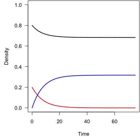<!-- --> --- # Susceptible-infected-recovered (SIR) model <video width="500" height="500" controls="controls" loop> <source src="Wk11_Disease_files/SIR.mp4" type="video/mp4"> </video> --- # Nice model, Chris, but how'bout those data? <div class="figure" style="text-align: center"> <img src="Wk11_Disease_files/Plague.jpg" alt=" " width="49%" /><img src="Wk11_Disease_files/Flu.jpg" alt=" " width="49%" /> <p class="caption"> </p> </div>